🎯 Semantic Entropy

This demo illustrates a state-of-the-art uncertainty quantification (UQ) approach known as semantic entropy. The token-probability-based semantic entropy method combines elements of black-box UQ (which generates multiple responses from the same prompt) and white-box UQ (which uses token probabilities of those generated responses) to compute entropy values and associated confidence scores. The discrete semantic entropy method is similar but functions solely as a black-box UQ method, as it does not require token probabilities. Both methods were proposed by Farquhar et al. (2024) and are demonstrated in this notebook.

📊 What You’ll Do in This Demo

1

Set up LLM and prompts.

Set up LLM instance and load example data prompts.

2

Generate LLM Responses and Confidence Scores

Generate and score LLM responses to the example questions using the SemanticEntropy() class.

3

Evaluate Hallucination Detection Performance

Visualize model accuracy at different thresholds of the semantic entropy-based confidence scores. Compute precision, recall, and F1-score of hallucination detection.

⚖️ Advantages & Limitations

Pros

• Universal Compatibility: Works with any LLM

• Intuitive: Easy to understand and implement

• No Internal Access Required: Doesn’t need token probabilities or model internals

Cons

• Higher Cost: Requires multiple generations per prompt

• Slower: Multiple generations and comparison calculations increase latency

import numpy as np
from sklearn.metrics import precision_score, recall_score, f1_score

from uqlm.utils import load_example_dataset, math_postprocessor, plot_model_accuracies, Tuner
from uqlm import SemanticEntropy

## 1. Set up LLM and Prompts

In this demo, we will illustrate this approach using a set of math questions from the gsm8k benchmark). To implement with your use case, simply replace the example prompts with your data.

# Load example dataset (gsm8k)
gsm8k = load_example_dataset("gsm8k", n=200)
gsm8k.head()

Loading dataset - gsm8k...
Processing dataset...
Dataset ready!

	question	answer
0	Natalia sold clips to 48 of her friends in Apr...	72
1	Weng earns $12 an hour for babysitting. Yester...	10
2	Betty is saving money for a new wallet which c...	5
3	Julie is reading a 120-page book. Yesterday, s...	42
4	James writes a 3-page letter to 2 different fr...	624

# Define prompts
MATH_INSTRUCTION = "When you solve this math problem only return the answer with no additional text.\n"
prompts = [MATH_INSTRUCTION + prompt for prompt in gsm8k.question]

In this example, we use AzureChatOpenAI to instantiate our LLM, but any LangChain Chat Model may be used. Be sure to replace with your LLM of choice.

# import sys
# !{sys.executable} -m pip install langchain-google-vertexai
from langchain_google_vertexai import ChatVertexAI

llm = ChatVertexAI(model="gemini-1.5-flash")

## 2. Generate responses and confidence scores

SemanticEntropy() - Generate LLM responses and compute consistency-based confidence scores for each response.

📋 Class Attributes

Parameter	Type & Default	Description
llm	BaseChatModeldefault=None	A langchain llm BaseChatModel. User is responsible for specifying temperature and other relevant parameters to the constructor of the provided llm object.
device	str or torch.devicedefault=”cpu”	Specifies the device that NLI model use for prediction. Only applies to ‘semantic_negentropy’, ‘noncontradiction’ scorers. Pass a torch.device to leverage GPU.
use_best	booldefault=True	Specifies whether to swap the original response for the uncertainty-minimized response among all sampled responses based on semantic entropy clusters. Only used if scorers includes ‘semantic_negentropy’ or ‘noncontradiction’.
system_prompt	str or Nonedefault=”You are a helpful assistant.”	Optional argument for user to provide custom system prompt for the LLM.
max_calls_per_min	intdefault=None	Specifies how many API calls to make per minute to avoid rate limit errors. By default, no limit is specified.
use_n_param	booldefault=False	Specifies whether to use n parameter for BaseChatModel. Not compatible with all BaseChatModel classes. If used, it speeds up the generation process substantially when num_responses is large.
postprocessor	callabledefault=None	A user-defined function that takes a string input and returns a string. Used for postprocessing outputs.
sampling_temperature	floatdefault=1	The ‘temperature’ parameter for LLM model to generate sampled LLM responses. Must be greater than 0.
nli_model_name	strdefault=”microsoft/deberta-large-mnli”	Specifies which NLI model to use. Must be acceptable input to AutoTokenizer.from_pretrained() and AutoModelForSequenceClassification.from_pretrained().
max_length	intdefault=2000	Specifies the maximum allowed string length for LLM responses for NLI computation. Responses longer than this value will be truncated in NLI computations to avoid OutOfMemoryError.

🔍 Parameter Groups

🧠 LLM-Specific

• llm

• system_prompt

• sampling_temperature

📊 Confidence Scores

• nli_model_name

• use_best

• postprocessor

🖥️ Hardware

• device

⚡ Performance

• max_calls_per_min

• use_n_param

💻 Usage Examples

# Basic usage with default parameters
se = SemanticEntropy(llm=llm)

# Using GPU acceleration, default scorers
se = SemanticEntropy(llm=llm, device=torch.device("cuda"))

# High-throughput configuration with rate limiting
se = SemanticEntropy(llm=llm, max_calls_per_min=200, use_n_param=True)

import torch

# Set the torch device
if torch.cuda.is_available():  # NVIDIA GPU
    device = torch.device("cuda")
elif torch.backends.mps.is_available():  # macOS
    device = torch.device("mps")
else:
    device = torch.device("cpu")  # CPU
print(f"Using {device.type} device")

Using cuda device

se = SemanticEntropy(
    llm=llm,
    max_calls_per_min=1000,  # set value to avoid rate limit error
    device=device,  # use if GPU available
)

Some weights of the model checkpoint at microsoft/deberta-large-mnli were not used when initializing DebertaForSequenceClassification: ['config']
- This IS expected if you are initializing DebertaForSequenceClassification from the checkpoint of a model trained on another task or with another architecture (e.g. initializing a BertForSequenceClassification model from a BertForPreTraining model).
- This IS NOT expected if you are initializing DebertaForSequenceClassification from the checkpoint of a model that you expect to be exactly identical (initializing a BertForSequenceClassification model from a BertForSequenceClassification model).

🔄 Class Methods

Method	Description & Parameters
SemanticEntropy.generate_and_score	Generate LLM responses, sampled LLM (candidate) responses, and compute confidence scores for the provided prompts. Parameters: prompts - (list of str) A list of input prompts for the model. num_responses - (int, default=5) The number of sampled responses used to compute consistency. show_progress_bars - (bool, default=True) If True, displays a progress bar while generating and scoring responses. Returns: UQResult containing data (prompts, responses, sampled responses, and confidence scores) and metadata 💡 Best For: Complete end-to-end uncertainty quantification when starting with prompts.
SemanticEntropy.score	Compute confidence scores on provided LLM responses. Should only be used if responses and sampled responses are already generated. Parameters: responses - (list of str) A list of LLM responses for the prompts. sampled_responses - (list of list of str) A list of lists of sampled LLM responses for each prompt. These will be used to compute consistency scores by comparing to the corresponding response from responses. show_progress_bars - (bool, default=True) If True, displays a progress bar while scoring responses. Returns: UQResult containing data (responses, sampled responses, and confidence scores) and metadata 💡 Best For: Computing uncertainty scores when responses are already generated elsewhere.

results = await se.generate_and_score(prompts=prompts, num_responses=10)

# # alternative approach: directly score if responses already generated
# results = se.score(responses=responses, sampled_responses=sampled_responses)

The LLM instance used here returns token probabilities during the response generation. In such scenario, SemanticEntropy class computes response probabilty in two ways: 1) Discrete semantic entropy: Equal probability to each response cluster and 2) Token-probability-based semantic entropy: Uses token probability to compute probability of each response cluster.

result_df = results.to_df()
result_df.head(5)

	response	discrete_entropy_value	discrete_confidence_score	sampled_responses	prompt	tokenprob_entropy_value	tokenprob_confidence_score
0	72\n	0.000000	1.000000	[72\n, 72\n, 72\n, 72\n, 72\n, 72\n, 72\n, 72\...	When you solve this math problem only return t...	0.000000	1.000000
1	$10\n	0.000000	1.000000	[$10\n, $10\n, $10\n, $10\n, $10\n, $10\n, $10...	When you solve this math problem only return t...	0.000000	1.000000
2	25\n	0.474139	0.802269	[25\n, 25\n, 25\n, 25\n, 25\n, 25\n, 25\n, 35\...	When you solve this math problem only return t...	0.080509	0.966425
3	30\n	0.474139	0.802269	[30\n, 36\n, 30\n, 36\n, 30\n, 30\n, 30\n, 30\...	When you solve this math problem only return t...	0.092084	0.961598
4	156\n	0.994924	0.585085	[156\n, 780\n, 312\n, 312\n, 156\n, 156\n, 156...	When you solve this math problem only return t...	0.646899	0.730222

## 3. Evaluate Hallucination Detection Performance

To evaluate hallucination detection performance, we ‘grade’ the responses against an answer key. Note the math_postprocessor is specific to our use case (math questions). If you are using your own prompts/questions, update the grading method accordingly.

# Populate correct answers and grade responses
result_df["answer"] = gsm8k.answer
result_df["response_correct"] = [math_postprocessor(r) == a for r, a in zip(result_df["response"], gsm8k["answer"])]
result_df.head(5)

	response	discrete_entropy_value	discrete_confidence_score	sampled_responses	prompt	tokenprob_entropy_value	tokenprob_confidence_score	answer	response_correct
0	72\n	0.000000	1.000000	[72\n, 72\n, 72\n, 72\n, 72\n, 72\n, 72\n, 72\...	When you solve this math problem only return t...	0.000000	1.000000	72	True
1	$10\n	0.000000	1.000000	[$10\n, $10\n, $10\n, $10\n, $10\n, $10\n, $10...	When you solve this math problem only return t...	0.000000	1.000000	10	True
2	25\n	0.474139	0.802269	[25\n, 25\n, 25\n, 25\n, 25\n, 25\n, 25\n, 35\...	When you solve this math problem only return t...	0.080509	0.966425	5	False
3	30\n	0.474139	0.802269	[30\n, 36\n, 30\n, 36\n, 30\n, 30\n, 30\n, 30\...	When you solve this math problem only return t...	0.092084	0.961598	42	False
4	156\n	0.994924	0.585085	[156\n, 780\n, 312\n, 312\n, 156\n, 156\n, 156...	When you solve this math problem only return t...	0.646899	0.730222	624	False

print(f"""Baseline LLM accuracy: {np.mean(result_df["response_correct"])}""")

Baseline LLM accuracy: 0.37

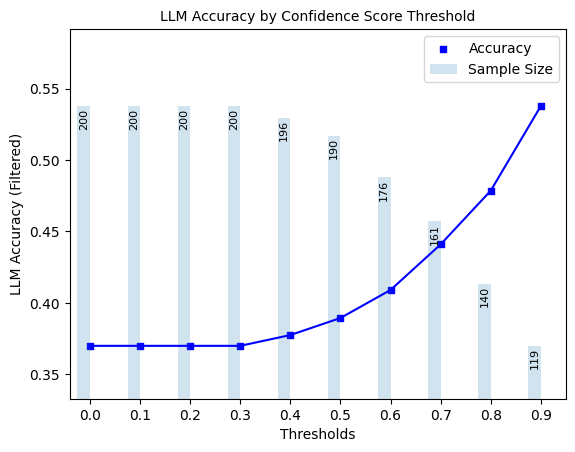
3.1 Filtered LLM Accuracy Evaluation

Here, we explore ‘filtered accuracy’ as a metric for evaluating the performance of our confidence scores. Filtered accuracy measures the change in LLM performance when responses with confidence scores below a specified threshold are excluded. By adjusting the confidence score threshold, we can observe how the accuracy of the LLM improves as less certain responses are filtered out.

We will plot the filtered accuracy across various confidence score thresholds to visualize the relationship between confidence and LLM accuracy. This analysis helps in understanding the trade-off between response coverage (measured by sample size below) and LLM accuracy, providing insights into the reliability of the LLM’s outputs.

Discrete Semantic Entropy

# Discrete Semantic Entropy
plot_model_accuracies(scores=result_df.discrete_confidence_score, correct_indicators=result_df.response_correct)

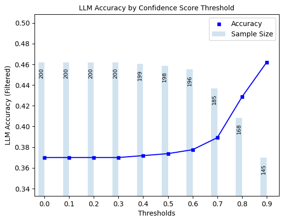
Discrete Semantic Entropy

plot_model_accuracies(scores=result_df.tokenprob_confidence_score, correct_indicators=result_df.response_correct)

3.2 Precision, Recall, F1-Score of Hallucination Detection

Lastly, we compute the optimal threshold for binarizing confidence scores, using F1-score as the objective. Using these thresholds, we compute precision, recall, and F1-score for our two semantic entropy-based scorer predictions of whether responses are correct.

# instantiate UQLM tuner object for threshold selection
split = len(result_df) // 2
t = Tuner()

correct_indicators = (result_df.response_correct) * 1  # Whether responses is actually correct
metric_values = {"Precision": [], "Recall": [], "F1-score": []}
optimal_thresholds = []
for confidence_score in ["discrete_confidence_score", "tokenprob_confidence_score"]:
    # tune threshold on first half
    y_scores = result_df[confidence_score]
    y_scores_tune = y_scores[0:split]
    y_true_tune = correct_indicators[0:split]
    best_threshold = t.tune_threshold(y_scores=y_scores_tune, correct_indicators=y_true_tune, thresh_objective="fbeta_score")

    y_pred = [(s > best_threshold) * 1 for s in y_scores]  # predicts whether response is correct based on confidence score
    optimal_thresholds.append(best_threshold)

    # evaluate on last half
    y_true_eval = correct_indicators[split:]
    y_pred_eval = y_pred[split:]
    metric_values["Precision"].append(precision_score(y_true=y_true_eval, y_pred=y_pred_eval))
    metric_values["Recall"].append(recall_score(y_true=y_true_eval, y_pred=y_pred_eval))
    metric_values["F1-score"].append(f1_score(y_true=y_true_eval, y_pred=y_pred_eval))

# print results
header = f"{'Metrics':<25}" + "".join([f"{scorer_name:<35}" for scorer_name in ["discrete_confidence_score", "tokenprob_confidence_score"]])
print("=" * len(header) + "\n" + header + "\n" + "-" * len(header))
for metric in metric_values.keys():
    print(f"{metric:<25}" + "".join([f"{round(x_, 3):<35}" for x_ in metric_values[metric]]))
print("-" * len(header))
print(f"{'F-1 optimal threshold':<25}" + "".join([f"{round(x_, 3):<35}" for x_ in optimal_thresholds]))
print("=" * len(header))

===============================================================================================
Metrics                  discrete_confidence_score          tokenprob_confidence_score
-----------------------------------------------------------------------------------------------
Precision                0.621                              0.6
Recall                   0.9                                0.9
F1-score                 0.735                              0.72
-----------------------------------------------------------------------------------------------
F-1 optimal threshold    0.88                               0.99
===============================================================================================

4. Scorer Definitions

Below are the definitions of the two confidence scores used in this demo.

Normalized Semantic Negentropy (Discrete)

Normalized Semantic Negentropy (NSN) normalizes the standard computation of discrete semantic entropy to be increasing with higher confidence and have [0,1] support. In contrast to the EMR and NCP, semantic entropy does not distinguish between an original response and candidate responses. Instead, this approach computes a single metric value on a list of responses generated from the same prompt. Under this approach, responses are clustered using an NLI model based on mutual entailment. We consider the discrete version of SE, where the final set of clusters is defined as follows:

:nbsphinx-math:`begin{equation}

SE(y_i; tilde{mathbf{y}}_i) = - sum_{C in mathcal{C}} P(C|y_i, tilde{mathbf{y}}_i)log P(C|y_i, tilde{mathbf{y}}_i),

end{equation}` where \(P(C|y_i, \tilde{\mathbf{y}}_i)\) denotes the probability a randomly selected response $y \in `{y_i} :nbsphinx-math:cup :nbsphinx-math:tilde{mathbf{y}}`_i $ belongs to cluster \(C\), and \(\mathcal{C}\) denotes the full set of clusters of \(\{y_i\} \cup \tilde{\mathbf{y}}_i\).

To ensure that we have a normalized confidence score with \([0,1]\) support and with higher values corresponding to higher confidence, we implement the following normalization to arrive at ormalized Semantic Negentropy (NSN): :nbsphinx-math:`begin{equation}

NSN(y_i; tilde{mathbf{y}}_i) = 1 - frac{SE(y_i; tilde{mathbf{y}}_i)}{log m},

end{equation}` where \(\log m\) is included to normalize the support.

Normalized Semantic Negentropy (Token-Probability-Based)

For this version, the formula is the same as above except \(P(C|y_i, \tilde{\mathbf{y}}_i)\) is computed using joint token probability.

© 2025 CVS Health and/or one of its affiliates. All rights reserved.

© 2025 CVS Health and/or one of its affiliates. All rights reserved.