🎯 White-Box Uncertainty Quantification

White-box Uncertainty Quantification (UQ) methods leverage token probabilities to estimate uncertainty. Multi-generation white-box methods generate multiple responses from the same prompt, combining the sampling approach of black-box UQ with token-probability-based singals. This demo provides an illustration of how to use state-of-the-art white-box UQ methods with uqlm. The following multi-generation scorers are available:

• Monte carlo sequence probability (Kuhn et al., 2023)

• Consistency and Confidence (CoCoA) (Vashurin et al., 2025)

• Semantic Negentropy (Farquhar et al., 2024)

• Semantic Density (Qiu et al., 2024)

• P(True) (Kadavath et al., 2022)

📊 What You’ll Do in This Demo

1

Set up LLM and prompts.

Set up LLM instance and load example data prompts.

2

Generate LLM Responses and Confidence Scores

Generate and score LLM responses to the example questions using the WhiteBoxUQ() class.

3

Evaluate Hallucination Detection Performance

Visualize model accuracy at different thresholds of the various white-box UQ confidence scores. Compute precision, recall, and F1-score of hallucination detection.

⚖️ Advantages & Limitations

Pros

• Robust Uncertainty Signals: Leverages token probabilities from multiple sampled responses.

• SOTA Performance: Enables use of top SOTA methods, including Semantic Entropy and Semantic Density.

Cons

• Limited Compatibility: Requires access to token probabilities, not available for all LLMs/APIs.

• Higher Cost: Requires multiple generations per prompt

• Slower: Multiple generations and comparison calculations increase latency

import numpy as np
from sklearn.metrics import precision_score, recall_score, f1_score

from uqlm import WhiteBoxUQ
from uqlm.utils import load_example_dataset, math_postprocessor, plot_model_accuracies, Tuner

## 1. Set up LLM and Prompts

In this demo, we will illustrate this approach using a set of math questions from the gsm8k benchmark. To implement with your use case, simply replace the example prompts with your data.

# Load example dataset (gsm8k)
gsm8k = load_example_dataset("gsm8k", n=100)
gsm8k.head()

Loading dataset - gsm8k...
Processing dataset...
Dataset ready!

	question	answer
0	Natalia sold clips to 48 of her friends in Apr...	72
1	Weng earns $12 an hour for babysitting. Yester...	10
2	Betty is saving money for a new wallet which c...	5
3	Julie is reading a 120-page book. Yesterday, s...	42
4	James writes a 3-page letter to 2 different fr...	624

# Define prompts
MATH_INSTRUCTION = "When you solve this math problem only return the answer with no additional text.\n"
prompts = [MATH_INSTRUCTION + prompt for prompt in gsm8k.question]

In this example, we use AzureChatOpenAI to instantiate our LLM, but any LangChain Chat Model may be used. Be sure to replace with your LLM of choice.

# import sys
# !{sys.executable} -m pip install python-dotenv
# !{sys.executable} -m pip install langchain-openai

# # User to populate .env file with API credentials. In this step, replace with your LLM of choice.
from dotenv import load_dotenv, find_dotenv
from langchain_openai import AzureChatOpenAI

load_dotenv(find_dotenv())
llm = AzureChatOpenAI(deployment_name="gpt-4o", openai_api_type="azure", openai_api_version="2024-02-15-preview", temperature=1)

## 2. Generate responses and confidence scores

WhiteBoxUQ() - Generate LLM responses and compute token-probability-based confidence scores for each response.

📋 Class Attributes

Parameter	Type & Default	Description
llm	BaseChatModeldefault=None	A langchain llm BaseChatModel. User is responsible for specifying temperature and other relevant parameters to the constructor of their llm object.
scorers	List[str]default=None	Specifies which white-box UQ scorers to include. Must be subset of [“normalized_probability”, “min_probability”, “sequence_probability”, “max_token_negentropy”, “mean_token_negentropy”, “probability_margin”, “monte_carlo_negentropy”, “consistency_and_confidence”, “semantic_negentropy”, “semantic_density”, “p_true”]. If None, defaults to [“normalized_probability”, “min_probability”].
system_prompt	str or Nonedefault=”You are a helpful assistant.”	Optional argument for user to provide custom system prompt for the LLM.
max_calls_per_min	intdefault=None	Specifies how many API calls to make per minute to avoid rate limit errors. By default, no limit is specified.
sampling_temperature	floatdefault=1	The ‘temperature’ parameter for LLM to use when generating sampled LLM responses. Only applies to “monte_carlo_negentropy”, “consistency_and_confidence”, “semantic_negentropy”, “semantic_density”. Must be greater than 0.

🔍 Parameter Groups

🧠 Model-Specific

• llm

• system_prompt

• sampling_temperature

📊 Confidence Scores

• scorers

⚡ Performance

• max_calls_per_min

wbuq = WhiteBoxUQ(
    llm=llm,
    scorers=[
        "monte_carlo_probability",  # requires multiple sampled responses per prompt
        "consistency_and_confidence",  # requires multiple sampled responses per prompt
        "p_true",  # generates one additional response per prompt, acts as logprobs-based self-judge
    ],
    max_calls_per_min=125,
)

🔄 Class Methods

Method	Description & Parameters
WhiteBoxUQ.generate_and_score	Generate LLM responses and compute confidence scores for the provided prompts. Parameters: prompts - (List[str] or List[List[BaseMessage]]) A list of input prompts for the model. num_responses - (int, default=5) The number of sampled responses to generate for sampling-based white-box UQ methods. Only applies to “monte_carlo_negentropy”, “consistency_and_confidence”, “semantic_negentropy”, “semantic_density”. show_progress_bars - (bool, default=True) If True, displays a progress bar while generating and scoring responses. Returns: UQResult containing data (prompts, responses, log probabilities, and confidence scores) and metadata 💡 Best For: Complete end-to-end uncertainty quantification when starting with prompts.
BlackBoxUQ.score	Compute confidence scores on provided LLM responses and logprobs. Should only be used if responses and sampled responses are already generated with logprobs. Parameters: responses - (List[str]) A list of LLM responses for the prompts. logprob_results - (List[List[str]]) A list of dictionaries, each returned by BaseChatModel.agenerate corresponding to responses. sampled_responses - (List[List[str]], default=None) A list of lists of sampled LLM responses for each prompt. Used to compute consistency scores by comparing to the corresponding response from responses. Required only for “monte_carlo_negentropy”, “consistency_and_confidence”, “semantic_negentropy”, “semantic_density” scorers. sampled_logprob_results - (List[List[str]], default=None) List of list of dictionaries, each returned by BaseChatModel.agenerate. These must correspond to sampled_responses. Required only for “monte_carlo_negentropy”, “consistency_and_confidence”, “semantic_negentropy”, “semantic_density” scorers. prompts - (List[List[str]], default=None) List of prompts from which responses were generated. Required only for “p_true” scorer. show_progress_bars - (bool, default=True) If True, displays a progress bar while scoring responses. Returns: UQResult containing data (responses, sampled responses, and confidence scores) and metadata 💡 Best For: Computing uncertainty scores when responses and logprobs are already generated elsewhere.

results = await wbuq.generate_and_score(prompts=prompts, num_responses=5)

result_df = results.to_df()
result_df.head()

	prompt	response	logprob	sampled_responses	sampled_logprob	consistency_and_confidence	monte_carlo_probability	p_true
0	When you solve this math problem only return t...	72	[{'token': '72', 'bytes': [55, 50], 'logprob':...	[72, 72, 72, 72, 72]	[[{'token': '72', 'bytes': [55, 50], 'logprob'...	0.999819	0.999955	0.377549
1	When you solve this math problem only return t...	$10	[{'token': '$', 'bytes': [36], 'logprob': -0.0...	[$10, $10, $10, $10, $10]	[[{'token': '$', 'bytes': [36], 'logprob': -0....	0.994463	0.994415	0.047430
2	When you solve this math problem only return t...	$20	[{'token': '$', 'bytes': [36], 'logprob': -0.0...	[$20, $20, $20, $20, $10]	[[{'token': '$', 'bytes': [36], 'logprob': -0....	0.923075	0.890358	0.777260
3	When you solve this math problem only return t...	48	[{'token': '48', 'bytes': [52, 56], 'logprob':...	[48, 48, 48, 48, 48]	[[{'token': '48', 'bytes': [52, 56], 'logprob'...	0.994755	0.996196	0.182436
4	When you solve this math problem only return t...	624	[{'token': '624', 'bytes': [54, 50, 52], 'logp...	[624, 624 pages., 624, 624, 624]	[[{'token': '624', 'bytes': [54, 50, 52], 'log...	0.954816	0.923305	0.981987

## 3. Evaluate Hallucination Detection Performance

To evaluate hallucination detection performance, we ‘grade’ the responses against an answer key. Note the math_postprocessor is specific to our use case (math questions). If you are using your own prompts/questions, update the grading method accordingly.

# Populate correct answers
result_df["answer"] = gsm8k.answer

# Grade responses against correct answers
result_df["response_correct"] = [math_postprocessor(r) == a for r, a in zip(result_df["response"], gsm8k["answer"])]
result_df.head(5)

	prompt	response	logprob	sampled_responses	sampled_logprob	consistency_and_confidence	monte_carlo_probability	p_true	answer	response_correct
0	When you solve this math problem only return t...	72	[{'token': '72', 'bytes': [55, 50], 'logprob':...	[72, 72, 72, 72, 72]	[[{'token': '72', 'bytes': [55, 50], 'logprob'...	0.999819	0.999955	0.377549	72	True
1	When you solve this math problem only return t...	$10	[{'token': '$', 'bytes': [36], 'logprob': -0.0...	[$10, $10, $10, $10, $10]	[[{'token': '$', 'bytes': [36], 'logprob': -0....	0.994463	0.994415	0.047430	10	True
2	When you solve this math problem only return t...	$20	[{'token': '$', 'bytes': [36], 'logprob': -0.0...	[$20, $20, $20, $20, $10]	[[{'token': '$', 'bytes': [36], 'logprob': -0....	0.923075	0.890358	0.777260	5	False
3	When you solve this math problem only return t...	48	[{'token': '48', 'bytes': [52, 56], 'logprob':...	[48, 48, 48, 48, 48]	[[{'token': '48', 'bytes': [52, 56], 'logprob'...	0.994755	0.996196	0.182436	42	False
4	When you solve this math problem only return t...	624	[{'token': '624', 'bytes': [54, 50, 52], 'logp...	[624, 624 pages., 624, 624, 624]	[[{'token': '624', 'bytes': [54, 50, 52], 'log...	0.954816	0.923305	0.981987	624	True

print(f"""Baseline LLM accuracy: {np.mean(result_df["response_correct"])}""")

Baseline LLM accuracy: 0.53

3.1 Filtered LLM Accuracy Evaluation

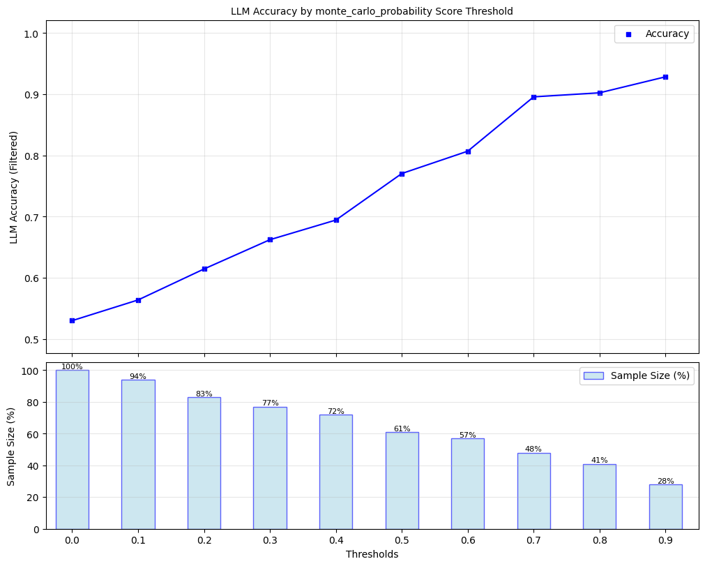
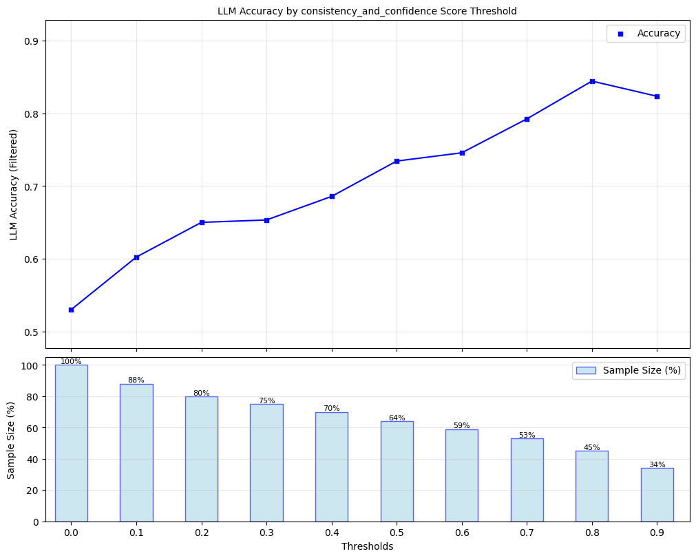
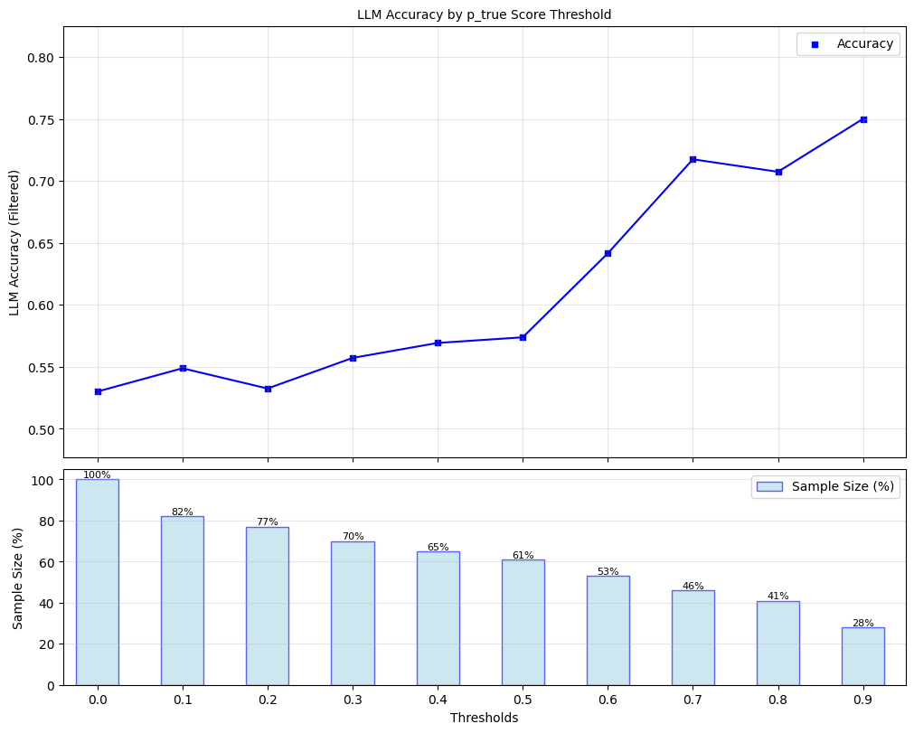
Here, we explore ‘filtered accuracy’ as a metric for evaluating the performance of our confidence scores. Filtered accuracy measures the change in LLM performance when responses with confidence scores below a specified threshold are excluded. By adjusting the confidence score threshold, we can observe how the accuracy of the LLM improves as less certain responses are filtered out.

We will plot the filtered accuracy across various confidence score thresholds to visualize the relationship between confidence and LLM accuracy. This analysis helps in understanding the trade-off between response coverage (measured by sample size below) and LLM accuracy, providing insights into the reliability of the LLM’s outputs. We conduct this analysis separately for each of our scorers.

for scorer in ["monte_carlo_probability", "consistency_and_confidence", "p_true"]:
    plot_model_accuracies(scores=result_df[scorer], correct_indicators=result_df.response_correct, title=f"LLM Accuracy by {scorer} Score Threshold", display_percentage=True)

3.2 Precision, Recall, F1-Score of Hallucination Detection

Lastly, we compute the optimal threshold for binarizing confidence scores, using F1-score as the objective. Using this threshold, we compute precision, recall, and F1-score for black box scorer predictions of whether responses are correct.

# instantiate UQLM tuner object for threshold selection
split = len(result_df) // 2
t = Tuner()

correct_indicators = (result_df.response_correct) * 1  # Whether responses is actually correct
metric_values = {"Precision": [], "Recall": [], "F1-score": []}
optimal_thresholds = []
for confidence_score in wbuq.scorers:
    # tune threshold on first half
    y_scores = result_df[confidence_score]
    y_scores_tune = y_scores[0:split]
    y_true_tune = correct_indicators[0:split]
    best_threshold = t.tune_threshold(y_scores=y_scores_tune, correct_indicators=y_true_tune, thresh_objective="fbeta_score")

    y_pred = [(s > best_threshold) * 1 for s in y_scores]  # predicts whether response is correct based on confidence score
    optimal_thresholds.append(best_threshold)

    # evaluate on last half
    y_true_eval = correct_indicators[split:]
    y_pred_eval = y_pred[split:]
    metric_values["Precision"].append(precision_score(y_true=y_true_eval, y_pred=y_pred_eval))
    metric_values["Recall"].append(recall_score(y_true=y_true_eval, y_pred=y_pred_eval))
    metric_values["F1-score"].append(f1_score(y_true=y_true_eval, y_pred=y_pred_eval))

# print results
header = f"{'Metrics':<30}" + "".join([f"{scorer_name:<30}" for scorer_name in wbuq.scorers])
print("=" * len(header) + "\n" + header + "\n" + "-" * len(header))
for metric in metric_values.keys():
    print(f"{metric:<30}" + "".join([f"{round(x_, 3):<30}" for x_ in metric_values[metric]]))
print("-" * len(header))
print(f"{'F-1 optimal threshold':<30}" + "".join([f"{round(x_, 3):<30}" for x_ in optimal_thresholds]))
print("=" * len(header))

========================================================================================================================
Metrics                       monte_carlo_probability       consistency_and_confidence    p_true
------------------------------------------------------------------------------------------------------------------------
Precision                     0.885                         0.909                         0.522
Recall                        0.885                         0.769                         0.923
F1-score                      0.885                         0.833                         0.667
------------------------------------------------------------------------------------------------------------------------
F-1 optimal threshold         0.64                          0.74                          0.02
========================================================================================================================

## 4. Scorer Definitions White-box UQ scorers leverage token probabilities of the LLM’s generated response to quantify uncertainty. All scorers have outputs ranging from 0 to 1, with higher values indicating higher confidence. We define several multi-generation white-box UQ scorers below.

Let the tokenization LLM response \(y_i\) be denoted as \(\{t_1,...,t_{L_i}\}\), where \(L_i\) denotes the number of tokens the response. Further, let \(y_1,...,y_m\) denote \(m\) sampled responses generated from the same prompt.

Monte Carlo Sequence Probability (monte_carlo_probability)

Monte Carlo Sequence Probability (MCSP) computes the average length-normalized sequence probability across sampled responses.

\[MCSP(y_1,y_2,...,y_m) = \frac{1}{m} \sum_{i=1}^m \prod_{t \in y_i} p_t^{\frac{1}{L_i}}\]

For more on this scorer, refer to Kuhn et al., 2023.

Consistency and Confidence Approach (CoCoA) (consistency_and_confidence)

Consistency and Confidence Approach (CoCoA) leverages two distinct signals: 1) similarity between an original response \(y_0\) and a set of sampled responses \(y_1,...,y_m\) and token probabilities from the original response \(y_0\).

We first get the length-normalized token probability of our original response:

\[LNTP(y_0) = \prod_{t \in y_0} p_t^{\frac{1}{L_0}}.\]

We then obtain average cosine similarity across pairings of the original response with all sampled responses, normalized to a [0,1] scale:

\[NCS(y_0; y_1,...,y_m) = \frac{1}{m} \sum_{i=1}^m \frac{\cos(y_0; y_i) + 1}{2}.\]

CoCoa is then calculated as the product of these two terms.

\[CoCoA(y_0; y_1,...,y_m) = LNTP(y_0) * NCS(y_0; y_1,...,y_m).\]

For more on this scorer, refer to Vashurin et al., 2025.

Normalized Semantic Negentropy

Normalized Semantic Negentropy (NSN) normalizes the standard computation of discrete semantic entropy to be increasing with higher confidence and have [0,1] support. Under this approach, responses are clustered using an NLI model based on mutual entailment. After obtaining the set of clusters \(\mathcal{C}\), semantic entropy is computed as:

\[SE(y_i; \tilde{\mathbf{y}}_i) = - \sum_{C \in \mathcal{C}} P(C|y_i, \tilde{\mathbf{y}}_i)\log P(C|y_i, \tilde{\mathbf{y}}_i),\]

where \(P(C|y_i, \tilde{\mathbf{y}}_i)\) is calculated as the average across response-level sequence probabilities (normalized or otherwise), and \(\mathcal{C}\) denotes the full set of clusters of \(\{y_i\} \cup \tilde{\mathbf{y}}_i\).

To ensure that we have a normalized confidence score with \([0,1]\) support and with higher values corresponding to higher confidence, we implement the following normalization to arrive at ormalized Semantic Negentropy (NSN):

\[NSN(y_i; \tilde{\mathbf{y}}_i) = 1 - \frac{SE(y_i; \tilde{\mathbf{y}}_i)}{\log m},\]

where \(\log m\) is included to normalize the support. For more on semantic entropy, refer to Farquhar et al., 2024; Kuhn et al., 2023, and for more on our normalized version, refer to Bouchard & Chauhan, 2025.

Semantic Density

Semantic Density (SD) approximates a probability density function (PDF) in semantic space for estimating response correctness. Given a prompt \(x\) with candidate response \(y_*\), the objective is to construct a PDF that assigns higher density to regions in the semantic space that correspond to correct responses. We begin by sampling \(M\) unique reference responses \(y_i\) (for \(i = 1, 2, \dots, M\)) conditioned on \(x\). For any pair of responses \(y_i, y_j\) with corresponding embeddings \(v_i, v_j\), the semantic distance is estimated as

\[\mathbb{E}(\Vert v_i,v_j \Vert^2) = p_c(y_i, y_j | x) + \dfrac{1}{2} \cdot p_n(y_i, y_j | x)\]

where \(p_c, p_n\) denote the contradiction and neutrality scores returned by a natural language inference (NLI) model, respectively. This estimated distance is incorporated in the kernel function \(K\) to smooth out the reference responses into a continuous distribution. The kernel function value can be obtained as

\[K(v_*, v_i) = (1 - \mathbb{E}(\Vert v_* - v_i \Vert^2))\mathbf{1}_{\mathbb{E}(\Vert v_* - v_i \Vert) \leq 1}\]

where \(\bf{1}\) is the indicator function such that \(\bf{1}_{\text{condition}} = 1\) when the condition holds and \(0\) otherwise. The final semantic density score is computed as

\[SD(y_* | x) = \dfrac{1}{\sum^M_{i=1}\sqrt[L_i]{p(y_i|x)}}\sum^M_{i=1}\sqrt[L_i]{p(y_i|x)}K(v_* - v_i)\]

where \(L_i\) denotes the length of \(y_i\).

P(True) (p_true)

The P(True) presents an LLM with a concatenation of a question and its own previous response. The LLM is asked to classify this statement as “True” or “False.” We derive this confidence score directly from the model’s token probability for answering “True” (or equivalently, 1-P(“False”) if the model answers “False”). For more on this scorer, refer to Kadavath et al., 2022.

© 2025 CVS Health and/or one of its affiliates. All rights reserved.